
Databricks Streaming: Part 1
Ingesting data using Auto Loader and Spark Structured Streaming

Griggs Reservoir Dam in Columbus, Ohio
Gone are the days of nightly batch executions and having to wait until the next day for refreshed data. With Spark and Databricks, you can process real-time data inexpensively, efficiently, and at scale with “set it and forget it” tools such as Auto Loader and Delta Live Tables. Real-time data ingestion is called “streaming” and is probably my favorite type of data source!
The most common use case for streaming is reading data from devices such as sensors or cameras. These devices can send measurements such as temperature and vibration to the cloud where it is picked up by tools such as Databricks to achieve real-time insights. This data is landed in a datalake and is valuable for all kinds of applications such as manufacturing, healthcare, or environmental science.
I wanted to give an example of how Streaming works in Databricks but needed a data source, and a colleague turned me onto the US Geological Survey Data. The USGS website has tons of constantly-updated data streams from all over the country. One of the services provided is Current Water Conditions. I was amazed to see the amount of sites being tracked by the USGS; almost every body of water in the country! This included the little reservoir on the Scioto River near my home in Columbus, Ohio.

Map of current streamflow (no pun intended) conditions from the USGS.
The USGS provides temperature and water-level readings for Griggs Reservoir every 15-60 minutes. This data is made available via a REST API endpoint that returns a JSON object containing the most recent readings. The USGS even provides a nifty tool that helps you construct the HTTP call needed to retrieve your data. If we call the API endpoint we can see how the boaters are faring this Memorial Day weekend:

As you can see, the JSON response contains a lot of information and can be hard to read. But we can pick out that the water at Griggs Reservoir was 18.5 degrees Celsius or about 65 degrees Fahrenheit at 9:00 AM this morning (pretty chilly!). It is typical to see streaming data in JSON format, particularly if it comes from devices. That is why it’s important to parse and transform the response using Databricks to get the information we need. But first, we need to automate this API call and land it in the “bronze” zone of the datalake (see here for more information on the medallion architecture).
There are several mechanisms for automating API calls, and in a true business scenario, you could have hundreds of devices sending data to an event ingestor such as Azure Event Hub before that data is streamed into the Databricks platform. But for a small example such as this, we can mimic the streaming source by performing the API call in a notebook, and scheduling the notebook to retrieve the data once every hour. I wrapped the API call in a Python function which overwrites the raw JSON in the datalake each time it runs. I am also pulling the last 12 hours of data every hour, that way any changes to the source measurements are accounted for.

Notebooks can be easily scheduled in Databricks.
Then, I created a second notebook that uses Auto Loader to pick up the raw JSON and append it to a Delta Table in the datalake. Auto Loader is an extension of Spark Structured Streaming that automatically detects when files are changed in the datalake and it’s the perfect tool for a “near real-time” scenario like this where we are working with “micro-batches”. The Delta Table will grow with each execution, and will likely contain duplicates since we are pulling the previous 12 hours each time. For this reason, I was sure to add a watermark that represents the timestamp of each execution.


Auto Loader appends raw data to Bronze Delta Table.
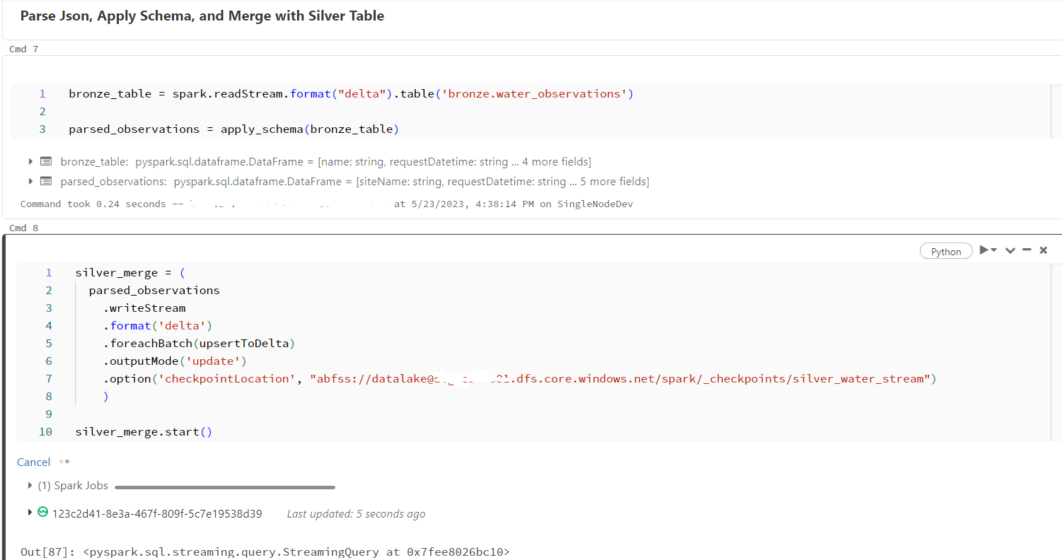
In the same notebook, I added a second stream that reads the data from the bronze table, parses the nested objects, applies a schema, and returns only the values that we need. This data is then written to the “silver” layer of the datalake in Delta format. In this step, the data is cleansed and then a merge operation is performed. The merge takes care of the duplicates by inserting new records into the table, and updating existing records with the latest values. I defined a couple functions for this portion of the notebook and added them to the streaming query to help with the data operations.

Once the setup is complete, all that’s left to do is start the stream by executing the notebook. While the stream is running and “listening” for changes to the data, the cluster will always be on. I chose a single-node cluster in Databricks to keep costs down since we’re dealing with such a small amount of data. While the stream is running, all we have to do is sit back and watch our cleansed data get written to the silver table!

In part 2, I will discuss moving the data from the “silver” zone to the “gold” zone using Delta Live Tables. Delta Live tables are a great feature of Databricks that allow you to automate the movement of data through the datalake zones with a visual interface. Once populated, the gold zone can be used to create up-to-date visuals and perform deeper analysis of the water data.